Techniques for Training Large Neural Networks

Large neural networks are at the core of many recent advances in AI, but training them is a difficult engineering and research challenge which requires orchestrating a cluster of GPUs to perform a single synchronized calculation. As cluster and model sizes have grown, machine learning practitioners have developed an increasing variety of techniques to parallelize model training over many GPUs. At first glance, understanding these parallelism techniques may seem daunting, but with only a few assumptions about the structure of the computation these techniques become much more clear—at that point, you’re just shuttling around opaque bits from A to B like a network switch shuttles around packets.


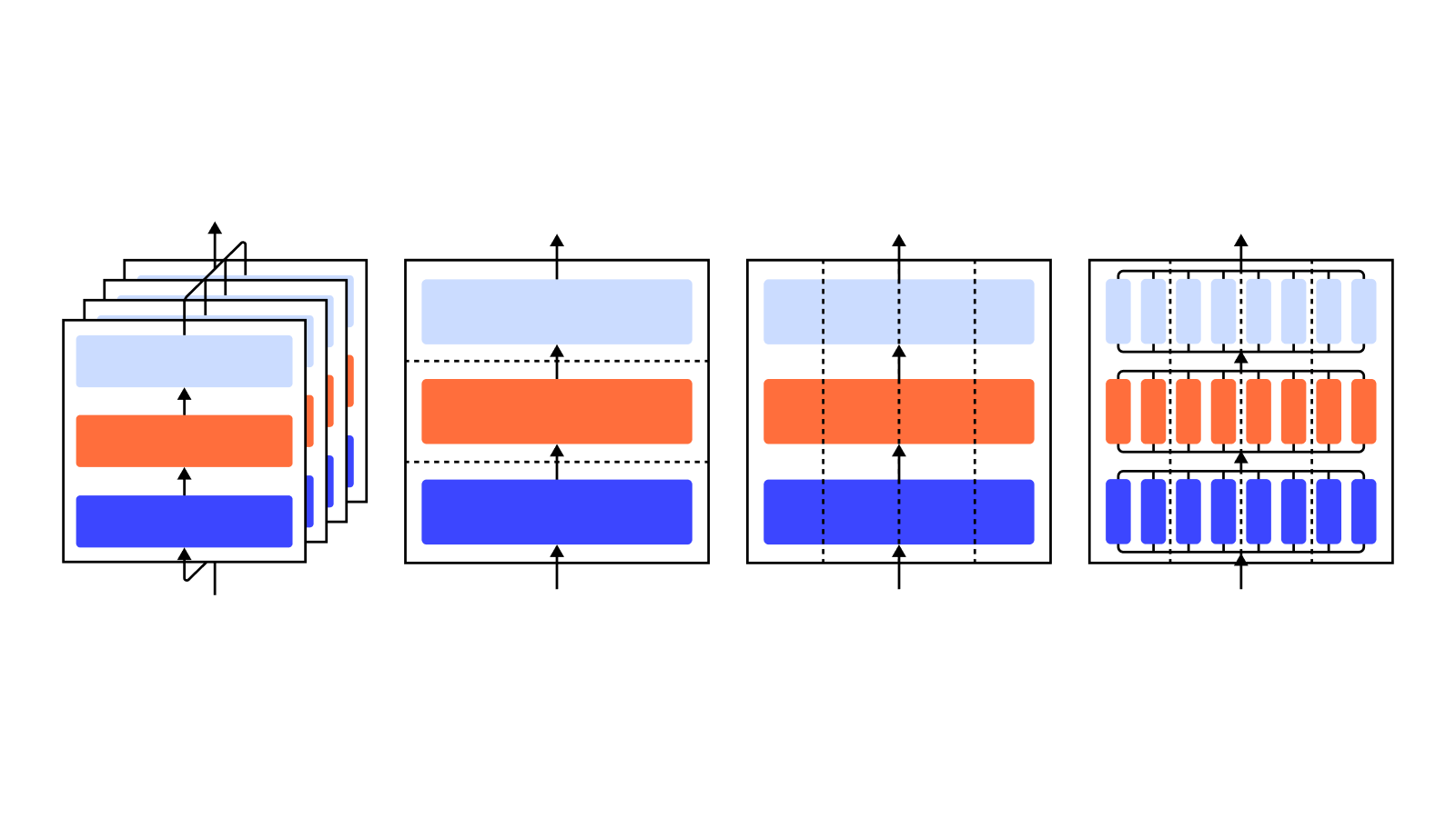
An illustration of various parallelism strategies on a three-layer model. Each color refers to one layer and dashed lines separate different GPUs.
No Parallelism
Training a neural network is an iterative process. In every iteration, we do a pass forward through a model’s layers to compute an output for each training example in a batch of data. Then another pass proceeds backward through the layers, propagating how much each parameter affects the final output by computing a gradient with respect to each parameter. The average gradient for the batch, the parameters, and some per-parameter optimization state is passed to an optimization algorithm, such as Adam, which computes the next iteration’s parameters (which should have slightly better performance on your data) and new per-parameter optimization state. As the training iterates over batches of data, the model evolves to produce increasingly accurate outputs.
Various parallelism techniques slice this training process across different dimensions, including:
- Data parallelism—run different subsets of the batch on different GPUs;
- Pipeline parallelism—run different layers of the model on different GPUs;
- Tensor parallelism—break up the math for a single operation such as a matrix multiplication to be split across GPUs;
- Mixture-of-Experts—process each example by only a fraction of each layer.
(In this post, we’ll assume that you are using GPUs to train your neural networks, but the same ideas apply to those using any other neural network accelerator.)
Data Parallelism
Data Parallel training means copying the same parameters to multiple GPUs (often called “workers”) and assigning different examples to each to be processed simultaneously. Data parallelism alone still requires that your model fits into a single GPU’s memory, but lets you utilize the compute of many GPUs at the cost of storing many duplicate copies of your parameters. That being said, there are strategies to increase the effective RAM available to your GPU, such as temporarily offloading parameters to CPU memory between usages.
As each data parallel worker updates its copy of the parameters, they need to coordinate to ensure that each worker continues to have similar parameters. The simplest approach is to introduce blocking communication between workers: (1) independently compute the gradient on each worker; (2) average the gradients across workers; and (3) independently compute the same new parameters on each worker. Step (2) is a blocking average which requires transferring quite a lot of data (proportional to the number of workers times the size of your parameters), which can hurt your training throughput. There are various asynchronous synchronization schemes to remove this overhead, but they hurt learning efficiency; in practice, people generally stick with the synchronous approach.
Pipeline Parallelism
With Pipeline Parallel training, we partition sequential chunks of the model across GPUs. Each GPU holds only a fraction of parameters, and thus the same model consumes proportionally less memory per GPU.
It’s straightforward to split a large model into chunks of consecutive layers. However, there’s a sequential dependency between inputs and outputs of layers, so a naive implementation can lead to a large amount of idle time while a worker waits for outputs from the previous machine to be used as its inputs. These waiting time chunks are known as “bubbles,” wasting the computation that could be done by the idling machines.

Forward

Backward

Gradient update

Idle

Illustration of a naive pipeline parallelism setup where the model is vertically split into 4 partitions by layer. Worker 1 hosts model parameters of the first layer of the network (closest to the input), while worker 4 hosts layer 4 (which is closest to the output). “F”, “B”, and “U” represent forward, backward and update operations, respectively. The subscripts indicate on which worker an operation runs. Data is processed by one worker at a time due to the sequential dependency, leading to large “bubbles” of idle time.
We can reuse the ideas from data parallelism to reduce the cost of the bubble by having each worker only process a subset of data elements at one time, allowing us to cleverly overlap new computation with wait time. The core idea is to split one batch into multiple microbatches; each microbatch should be proportionally faster to process and each worker begins working on the next microbatch as soon as it’s available, thus expediting the pipeline execution. With enough microbatches the workers can be utilized most of the time with a minimal bubble at the beginning and end of the step. Gradients are averaged across microbatches, and updates to the parameters happen only once all microbatches have been completed.
The number of workers that the model is split over is commonly known as pipeline depth.
During the forward pass, workers only need to send the output (called activations) of its chunk of layers to the next worker; during the backward pass, it only sends the gradients on those activations to the previous worker. There’s a big design space of how to schedule these passes and how to aggregate the gradients across microbatches. GPipe has each worker process forward and backward passes consecutively and then aggregates gradients from multiple microbatches synchronously at the end. PipeDream instead schedules each worker to alternatively process forward and backward passes.

Forward

Backward

Update

Idle
GPipe
PipeDream

Comparison of GPipe and PipeDream pipelining schemes, using 4 microbatches per batch. Microbatches 1-8 correspond to two consecutive data batches. In the image, “(number)” indicates on which microbatch an operation is performed and the subscript marks the worker ID. Note that PipeDream gets more efficiency by performing some computations with stale parameters.
Tensor Parallelism
Pipeline parallelism splits a model “vertically” by layer. It’s also possible to “horizontally” split certain operations within a layer, which is usually called Tensor Parallel training. For many modern models (such as the Transformer), the computation bottleneck is multiplying an activation batch matrix with a large weight matrix. Matrix multiplication can be thought of as dot products between pairs of rows and columns; it’s possible to compute independent dot products on different GPUs, or to compute parts of each dot product on different GPUs and sum up the results. With either strategy, we can slice the weight matrix into even-sized “shards”, host each shard on a different GPU, and use that shard to compute the relevant part of the overall matrix product before later communicating to combine the results.
One example is Megatron-LM, which parallelizes matrix multiplications within the Transformer’s self-attention and MLP layers. PTD-P uses tensor, data, and pipeline parallelism; its pipeline schedule assigns multiple non-consecutive layers to each device, reducing bubble overhead at the cost of more network communication.
Sometimes the input to the network can be parallelized across a dimension with a high degree of parallel computation relative to cross-communication. Sequence parallelism is one such idea, where an input sequence is split across time into multiple sub-examples, proportionally decreasing peak memory consumption by allowing the computation to proceed with more granularly-sized examples.
Mixture-of-Experts (MoE)
With the Mixture-of-Experts (MoE) approach, only a fraction of the network is used to compute the output for any one input. One example approach is to have many sets of weights and the network can choose which set to use via a gating mechanism at inference time. This enables many more parameters without increased computation cost. Each set of weights is referred to as “experts,” in the hope that the network will learn to assign specialized computation and skills to each expert. Different experts can be hosted on different GPUs, providing a clear way to scale up the number of GPUs used for a model.

Illustration of a mixture-of-experts (MoE) layer. Only 2 out of the n experts are selected by the gating network. (Image adapted from: Shazeer et al., 2017)
GShard scales an MoE Transformer up to 600 billion parameters with a scheme where only the MoE layers are split across multiple TPU devices and other layers are fully duplicated. Switch Transformer scales model size to trillions of parameters with even higher sparsity by routing one input to a single expert.
Other Memory Saving Designs
There are many other computational strategies to make training increasingly large neural networks more tractable. For example:
-
To compute the gradient, you need to have saved the original activations, which can consume a lot of device RAM. Checkpointing (also known as activation recomputation) stores any subset of activations, and recomputes the intermediate ones just-in-time during the backward pass. This saves a lot of memory at the computational cost of at most one additional full forward pass. One can also continually trade off between compute and memory cost by selective activation recomputation, which is checkpointing subsets of the activations that are relatively more expensive to store but cheaper to compute.
-
Mixed Precision Training is to train models using lower-precision numbers (most commonly FP16). Modern accelerators can reach much higher FLOP counts with lower-precision numbers, and you also save on device RAM. With proper care, the resulting model can lose almost no accuracy.
-
Offloading is to temporarily offload unused data to the CPU or amongst different devices and later read it back when needed. Naive implementations will slow down training a lot, but sophisticated implementations will pre-fetch data so that the device never needs to wait on it. One implementation of this idea is ZeRO which splits the parameters, gradients, and optimizer states across all available hardware and materializes them as needed.
-
Memory Efficient Optimizers have been proposed to reduce the memory footprint of the running state maintained by the optimizer, such as Adafactor.
-
Compression also can be used for storing intermediate results in the network. For example, Gist compresses activations that are saved for the backward pass; DALL·E compresses the gradients before synchronizing them.
At OpenAI, we are training and improving large models from the underlying infrastructure all the way to deploying them for real-world problems. If you’d like to put the ideas from this post into practice—especially relevant for our Scaling and Applied Research teams—we’re hiring!
Go to Source
Author: Lilian Weng
https://openai.com/blog/techniques-for-training-large-neural-networks/


